# Temporal Compositing and Provenance {#sec-temporal-compositing}
---
jupyter: ds-flood-gfm
---
Individual satellite observations have coverage gaps --- areas where no Sentinel-1 pass overlapped on a given day. To produce a gap-free flood map, we combine observations across multiple days. This chapter explains the compositing strategies and the provenance tracking system that records which observation date each pixel came from.
```{python}
import matplotlib.pyplot as plt
from matplotlib.colors import ListedColormap, BoundaryNorm
import matplotlib.patches as mpatches
import numpy as np
import geopandas as gpd
from fsspec.implementations.http import HTTPFileSystem
import ocha_stratus as stratus
from ds_flood_gfm.geo_utils import generate_rdylgn_colors

%matplotlib inline
plt.rcParams['figure.dpi'] = 100
```
```{python}
notebook_config = {
    'iso3': 'JAM',
    'start_date': '2025-10-20',
    'end_date': '2025-10-29',
}

GLOBAL_ADM1 = (
    "https://data.fieldmaps.io/edge-matched/humanitarian/intl/adm1_polygons.parquet"
)
filesystem = HTTPFileSystem()
filters = [("iso_3", "=", notebook_config['iso3'])]
gdf = gpd.read_parquet(GLOBAL_ADM1, filesystem=filesystem, filters=filters)
gdf_aoi = gdf.dissolve()
bbox = gdf_aoi.total_bounds
```
## Compositing Strategies
After querying STAC and building a lazy xarray stack (see @sec-querying-gfm), we group observations by day and apply one of two compositing modes.
### Daily Composites
Multiple Sentinel-1 passes can occur on the same day. We take the max value per day: flood (1) > no-flood (0) > nodata (NaN).
```{python}
#| eval: false
# Group by day and take the maximum flood value per day
stack_flood_max = stack_flood_clipped.groupby("time.date").max()
```
### The "Latest" Strategy: Forward-Fill
The `latest` mode fills gaps by carrying forward the most recent valid observation for each pixel. If a pixel was observed on day 3 but not day 5, it keeps the day-3 value. If re-observed on day 7 and no longer flooded, the day-7 value overwrites.
This is the operationally relevant mode --- it shows the **current best estimate** of flood extent.
```{python}
#| eval: false
ic_latest = stack_flood_max.ffill(dim="time")
latest_composite = ic_latest.isel(time=-1).compute()
```
### The "Cumulative" Strategy: Spatial Union
The `cumulative` mode takes the union of all observations --- any pixel that was ever flooded during the time window is marked as flooded. Useful for total impact assessment.
```{python}
#| eval: false
cumulative_composite = (stack_flood_max == 1).any(dim="time").compute()
```
## Provenance Raster
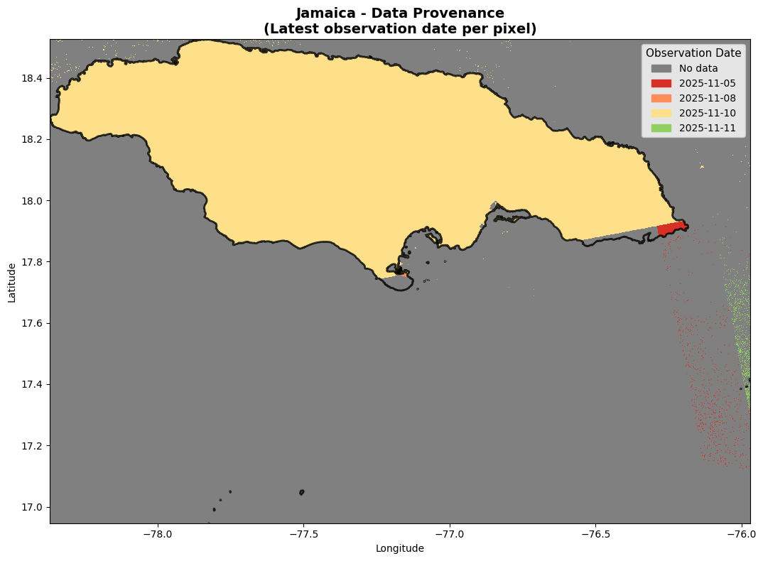
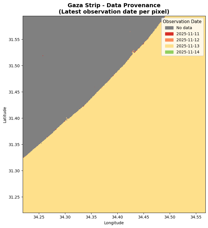
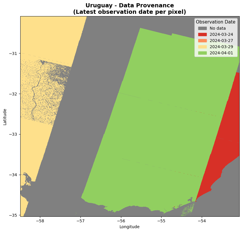
The provenance raster answers: **"which observation date does each pixel come from?"** This is critical for humanitarian reporting --- responders need to know how fresh the data is.
The algorithm:
1. For each pixel, find the **last** time step with valid data (using reversed `argmax`)
2. Encode as an integer index mapping to observation dates
3. Mask pixels that were never observed
```{python}
#| eval: false
from ds_flood_gfm.datasources.gfm import create_provenance_raster

# Create provenance raster (stays lazy until .compute())
provenance_idx, date_mapping = create_provenance_raster(stack_flood_max, unique_dates)
provenance_computed = provenance_idx.compute()
```
The result is a 2D raster where each pixel's value maps to a date, visualized with a red (oldest) to green (newest) colormap.
## Provenance Maps
Here we load pre-computed provenance rasters from blob storage. Each COG encodes integer date indices per pixel, and the filename contains the observation dates used.
```{python}
def plot_provenance_raster(blob_name, title, gdf_boundary=None, downsample=4):
    """
    Load a provenance COG from blob and render with RdYlGn colormap.
    Red = oldest observation, Green = most recent.
    """
    da_prov = stratus.open_blob_cog(blob_name, container_name="projects").squeeze(drop=True)
    data = da_prov.values
    bounds_rio = da_prov.rio.bounds()
    extent = [bounds_rio[0], bounds_rio[2], bounds_rio[1], bounds_rio[3]]

    # Parse dates from filename
    fname_parts = blob_name.split('/')[-1].split('_')
    date_strings = [p for p in fname_parts if len(p) == 8 and p.isdigit()]
    date_labels = [f"{d[:4]}-{d[4:6]}-{d[6:8]}" for d in date_strings]

    n_dates = len(date_labels)
    prov_colors = generate_rdylgn_colors(n_dates)

    # Build colormap: grey for no data, then RdYlGn date colors
    all_colors = ['grey'] + prov_colors
    prov_cmap = ListedColormap(all_colors)
    prov_bounds = [-1.5] + [i - 0.5 for i in range(n_dates + 1)]
    prov_norm = BoundaryNorm(prov_bounds, prov_cmap.N)

    data_viz = data.copy()
    if np.issubdtype(data.dtype, np.floating):
        data_viz = np.where(np.isnan(data_viz), -1, data_viz)
    data_viz = data_viz[::downsample, ::downsample]

    fig, ax = plt.subplots(1, 1, figsize=(14, 8))
    ax.imshow(data_viz, cmap=prov_cmap, norm=prov_norm,
              interpolation="nearest", origin="upper", extent=extent)

    if gdf_boundary is not None:
        gdf_boundary.boundary.plot(ax=ax, color="black", linewidth=2, alpha=0.8)

    ax.set_title(f"{title}\n(Latest observation date per pixel)",
                 fontsize=14, fontweight="bold")
    ax.set_xlabel("Longitude")
    ax.set_ylabel("Latitude")

    legend_patches = [mpatches.Patch(color='grey', label='No data')]
    for i, date in enumerate(date_labels):
        legend_patches.append(mpatches.Patch(color=prov_colors[i], label=date))
    ax.legend(handles=legend_patches, loc='upper right', title='Observation Date',
              fontsize=10, title_fontsize=11)

    plt.tight_layout()
    plt.show()
    return da_prov
```
### Jamaica — Hurricane Melissa
```{python}
da_jam = plot_provenance_raster(
    "ds-flood-gfm/processed/provenance_raster/JAM_20251105_20251108_20251110_20251111_nopop_cumulative_provenance.tif",
    title="Jamaica - Data Provenance",
    gdf_boundary=gdf_aoi,
)
```
### Gaza Strip
```{python}
da_gaza = plot_provenance_raster(
    "ds-flood-gfm/processed/provenance_raster/gaza_strip_adm1_20251111_20251112_20251113_20251114_nopop_cumulative_provenance.tif",
    title="Gaza Strip - Data Provenance",
)
```
### Uruguay
```{python}
da_ury = plot_provenance_raster(
    "ds-flood-gfm/processed/provenance_raster/URY_20240324_20240327_20240329_20240401_nopop_cumulative_provenance.tif",
    title="Uruguay - Data Provenance",
)
```
::: {.callout-tip}
## Rechunking for Temporal Operations
Operations like `ffill` and `argmax` along the time dimension require all timesteps to be in a single chunk. The library uses `chunk({'time': -1, 'y': 4096, 'x': 4096})` to consolidate the time dimension into one chunk while keeping spatial chunks manageable. This dramatically reduces the Dask task graph compared to the default chunking.
:::
## Library Functions
The `ds_flood_gfm.datasources.gfm` module wraps these operations into reusable functions:
- `query_gfm_stac(bbox, target_date, n_search)` --- queries the STAC API with bidirectional temporal scanning
- `create_flood_composite(items, bbox, n_images, mode)` --- builds the lazy stack, creates daily composites, applies the chosen compositing strategy
- `create_provenance_raster(stack_flood_max, unique_dates)` --- generates the provenance layer
The production scripts in @sec-production-pipeline use these functions to generate composites for any configured country with a single CLI call.