# Toward an Open-Source FloodScan? {#sec-downscaling-poc}
---
jupyter: ds-flood-gfm
---
FloodScan is a licensed product, but its pipeline is documented by its
authors. The Data Users Guide states it plainly: "FloodScan processing
produces an intermediate flooded fraction product at the passive microwave
satellite data scales (~22-km). The algorithm downscales flooded fraction to
make its flood depiction products (e.g., 90-m scale)" (FloodScan Data Users
Guide v05R01, AER 2021, §1.2). The downscaling database is described in
[Galantowicz (AER, AGU 2018)](https://ui.adsabs.harvard.edu/abs/2018AGUFM.H51B..03G/abstract)
as "built from topography, hydrology, and Global Surface Water Explorer
data"; the approach dates to Galantowicz 2002.
Every ingredient in that recipe has a free counterpart: GFDS supplies the
passive microwave signal (from the same instruments, posted at ~10 km rather
than ~22 km), and JRC Global Surface Water supplies the water-history
database. So this chapter takes an angle worth stating explicitly: **can we
build an open-source FloodScan?** And with a finer-resolution microwave
input and a 1998-to-present free archive, could it eventually be better?
The pipeline has two stages, because GFDS does not measure an amount of
water. It measures how *unusual* a pixel looks compared to its own history,
and you cannot draw "unusual" on a map at 90 m:
1. **Calibrate**: convert the GFDS reading into an estimated share of each
10 km pixel that is under water (a flooded fraction).
2. **Allocate**: split that share among the small (~83 m) cells inside each
pixel, marking the most flood-prone cells as flooded first. (Why the odd
83 m: the Landsat water map comes at ~28 m; we aggregate it 3×3 to
0.00075°, chosen because 0.09° divides by it exactly, so every GFDS pixel
holds a clean 120×120 block of fine cells. FloodScan's "90 m" is 3
arcseconds; ours is 2.7, the price of nesting into the GFDS grid.)
Stage 2 depends on what statisticians call a **prior**: information that
existed before today's satellite reading. Ours is a historical water map
built from every Landsat image since 1984: for each ~30 m cell, the share of
observations in which it was wet. River channels score near 100%, floodplains
somewhere in the tens, dry land zero. The division of labour is strict:
today's GFDS reading sets *how much* of each pixel is flooded, and the
historical map decides *which cells* get marked.
Full technical write-up:
[`docs/gfds-downscaling-poc.md`](https://github.com/OCHA-DAP/ds-flood-gfm/blob/main/docs/gfds-downscaling-poc.md);
code in `experiments/gfds_downscaling_poc/`.
## The methods, up front
Four different calibration methods appear in this chapter, and it matters
which figure uses which. Declared once, here:
| Label | Calibration method | Uses licensed data? | Role in this chapter |
|---|---|---|---|
| **R0** | Per-pixel lookup table trained on FloodScan SFED (rank matching between each pixel's GFDS and SFED histories) | **Yes**, trained on SFED | The *reproduction* test: how well can free input copy the licensed product? Also the ceiling for the independent methods. The downscaled-GFDS maps use the R0 fraction unless labelled otherwise; the allocation score table also includes the R1 chain. |
| **R1** | Physics: invert the wet/dry mixing equation with a literature emissivity contrast (K ≈ 0.35 at 36 GHz) and each pixel's own dry-season signal level | No | The *independence* test's lead candidate |
| **R2** | Per-pixel linear map anchored to the driest and wettest fractions Landsat ever observed (Global Surface Water) | No | Independence test, optical anchor |
| **R3** | Like R2 but the wet anchor is Sentinel-1 extent aggregated to the pixel for the October peak window | No | Independence test, radar anchor |
Equally important, the things that are **never calibration inputs, only
comparison points**:
- **FloodScan SFED**: the benchmark throughout. For R1, R2, R3 it is fully
external (they never see it), so agreement with it is evidence. For R0 it
is the training target, so agreement is partly by construction; R0's honest
scores come from held-out days its lookup tables never saw.
- **GFM Sentinel-1 radar**: a different product with a different overpass
cadence. It appears once, late, to arbitrate one narrow question about the
allocation stage. It calibrates nothing.
- **The history-only control**: an allocation map built with no 2022
satellite input at all, used to measure how much of the fine-scale map
comes from the historical prior rather than from any satellite.
The chapter now runs three tests in order: reproduction (R0 vs SFED),
independence (R1-R3 vs SFED), and allocation (the 83 m maps).
## Test 1: reproduction — the R0 lookup vs FloodScan
R0 is a per-pixel lookup table. For each 10 km pixel we line up its history
of GFDS readings against its history of FloodScan readings: a middling GFDS
day maps to that pixel's typical FloodScan value, an extreme day to an
extreme value. To keep ourselves honest, the table is built from half the
days (alternating) and every score below comes from the other half, days the
table never saw.
```{python}
#| eval: false
#| code-summary: "experiments/gfds_downscaling_poc/01_calibrate_fraction.py (method R0)"
{{< include ../experiments/gfds_downscaling_poc/01_calibrate_fraction.py >}}
```
```{python}
#| code-summary: "load POC results (fails loudly if the scripts haven't been run)"
from pathlib import Path

import matplotlib.pyplot as plt
import numpy as np
import pandas as pd
import xarray as xr

POC = next((p for p in (Path("outputs/gfds_downscaling_poc"),
                        Path("../outputs/gfds_downscaling_poc")) if p.exists()), None)
if POC is None or not (POC / "downscale_maps.npz").exists():
    raise FileNotFoundError(
        "POC outputs not found. Run experiments/gfds_downscaling_poc/ scripts "
        "01-07 from the repo root first (inputs are cached or range-read)."
    )
skill_cal = pd.read_csv(POC / "calibration_skill.csv", index_col=0)
frac = xr.open_dataarray(POC / "gfds_calibrated_fraction.nc")  # R0 fraction
sfed = xr.open_dataarray(POC / "sfed_on_gfds.nc")
skill_cal
```
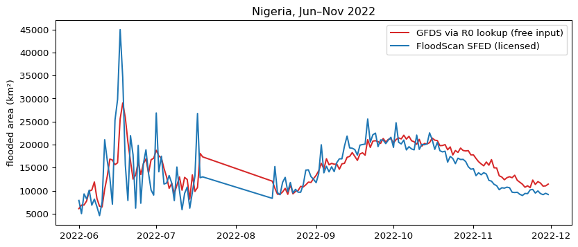
On the unseen days, R0 predicts FloodScan's value with a typical error of
0.040 (in flooded-share units, over pixels that actually flooded), versus
0.048 for the lazy strategy of always guessing each pixel's average. A
modest margin, honestly earned. The more tangible payoff is that GFDS can
now express something it never could before: how many square kilometres are
under water.
```{python}
#| fig-cap: "Flooded area per day over Nigeria. Red: fraction from the R0 lookup (free input, SFED-trained). Blue: licensed FloodScan SFED (here and in every comparison, resampled onto the GFDS 0.09° grid). At FloodScan's peak, the R0 estimate reaches 84% of its area."
px_km2 = (0.09 * 111.32) ** 2
both = np.isfinite(frac.values) & np.isfinite(sfed.values)
a_gfds = np.where(both, frac.values, 0).sum(axis=(1, 2)) * px_km2
a_sfed = np.where(both, sfed.values, 0).sum(axis=(1, 2)) * px_km2
fig, ax = plt.subplots(figsize=(10, 4))
ax.plot(frac.time, a_gfds, color="tab:red", label="GFDS via R0 lookup (free input)")
ax.plot(sfed.time, a_sfed, color="tab:blue", label="FloodScan SFED (licensed)")
ax.set_ylabel("flooded area (km²)")
ax.legend()
ax.set_title("Nigeria, Jun–Nov 2022")
plt.show()
```
```{python}
#| fig-cap: "CALIBRATION STAGE ONLY, 10 km grid, no downscaling. Mean flooded fraction 6-13 Oct 2022. Left: the R0 (SFED-trained) fraction from the free GFDS input. Right: licensed FloodScan SFED, resampled from its native 0.083° grid onto the GFDS 0.09° grid so the two fields compare cell by cell. Because R0 is trained on SFED (alternating days from this same season), close agreement here is partly by construction; the held-out-day scores above are the fair skill test."
#| fig-height: 5.5
peak = slice("2022-10-06", "2022-10-13")
wg = frac.sel(time=peak).mean("time")
ws = sfed.sel(time=peak).mean("time")
fig, axes = plt.subplots(1, 2, figsize=(13, 5.5), sharex=True, sharey=True)
wg.plot(ax=axes[0], vmin=0, vmax=0.5, cmap="Blues", add_colorbar=False)
axes[0].set_title("GFDS fraction via R0 lookup (free input)")
im = ws.plot(ax=axes[1], vmin=0, vmax=0.5, cmap="Blues", add_colorbar=False)
axes[1].set_title("FloodScan SFED (licensed)")
fig.colorbar(im, ax=axes, shrink=0.8, label="flooded fraction")
plt.show()

g, s = wg.values.ravel(), ws.values.ravel()
ok = np.isfinite(g) & np.isfinite(s)
wet = ok & ((g > 0.02) | (s > 0.02))
print(f"pixel correlation, all valid pixels: {np.corrcoef(g[ok], s[ok])[0,1]:.2f}")
print(f"pixel correlation, pixels either product calls wet (>2%): "
      f"{np.corrcoef(g[wet], s[wet])[0,1]:.2f} (n={int(wet.sum())})")
print(f"mean fraction over wet pixels: GFDS-R0 {g[wet].mean():.3f} "
      f"| FloodScan {s[wet].mean():.3f}")
```
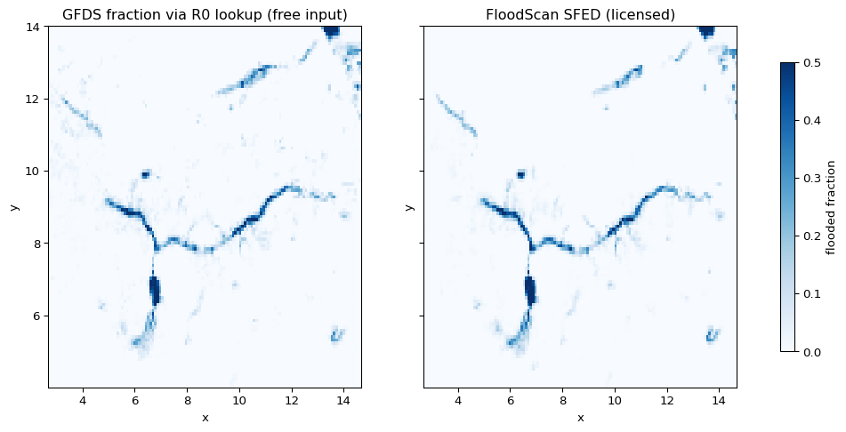
A note on why the left panel looks as crisp as the right one, when the raw
GFDS anomaly in @sec-alternative-sources looked visibly coarser. We measured
it, and the coarser look is mostly an optical effect, not a resolution
difference: the two fields have identical fine-scale smoothness on the
shared grid (one-cell spatial autocorrelation 0.74 for both season-max
fields). What differs is how much of each map is lit up. Sixty-one percent
of the GFDS anomaly map sits above a quarter of its color scale, against 7%
for SFED, because the anomaly carries low-level wet-season signal everywhere
while FloodScan's MDFF threshold blanks it. A mostly blank map with thin
features reads as sharp; a mostly colored map reads as blobby. The R0
conversion inherits SFED's per-pixel value ranges, which zero that
background out, so the converted map takes on SFED's sparse look. One real,
secondary difference survives the measurement: SFED's features stay
correlated further (0.58 vs 0.45 at two cells), reflecting the organized
corridors its hydrological database imposes.
## Test 2: independence — can we calibrate without FloodScan?
R0 proves the free input can copy the licensed product, but a copy is not an
independent product. AER did not have a reference product when they built
FloodScan; they got flooded fraction from brightness temperature with
physics: a partly flooded pixel's signal is a mix of a wet and a dry
component, and the mixing equation can be inverted. R1, R2, and R3 are three
ways to do that without touching FloodScan, which makes SFED a fully fair
external benchmark for them.
```{python}
#| eval: false
#| code-summary: "experiments/gfds_downscaling_poc/06_independent_fractions.py (methods R1, R2, R3)"
{{< include ../experiments/gfds_downscaling_poc/06_independent_fractions.py >}}
```
```{python}
#| fig-cap: "Flooded area over the confluence AOI: the three FloodScan-free calibrations (R1-R3), the SFED-trained ceiling (R0), and FloodScan itself. R1 (green) reproduces the flood wave and its peak with no FloodScan input; both anchor routes flatline because their anchors never saw a 2022-sized flood."
z2 = np.load(POC / "independent_fractions.npz")
R1, R2, R3, R0, W = (z2[k] for k in ("R1", "R2", "R3", "R0", "W"))
tt = pd.to_datetime(z2["time"])
pxa = (0.09 * 111.32) ** 2
okW = np.isfinite(W)
fig, ax = plt.subplots(figsize=(11, 4.5))
for P, lab, col in [(R1, "R1 physics", "tab:green"),
                    (R2, "R2 optical anchor", "tab:red"),
                    (R3, "R3 radar anchor", "tab:orange"),
                    (R0, "R0 SFED-trained (ceiling)", "tab:grey")]:
    okp = np.isfinite(P) & okW
    ax.plot(tt, np.nansum(np.where(okp, P, 0), axis=1) * pxa, label=lab,
            color=col, lw=1.2)
ax.plot(tt, np.nansum(np.where(okW, W, 0), axis=1) * pxa,
        label="FloodScan SFED (benchmark)", color="tab:blue", lw=2)
ax.set_ylabel("flooded area (km²)")
ax.legend(fontsize=8)
plt.show()

wet_cells = z2["wet_cells"]
def rscore(P):
    m = np.isfinite(P) & np.isfinite(W) & wet_cells[None, :]
    a_p = np.nansum(np.where(np.isfinite(P) & okW, P, 0), axis=1)
    a_w = np.nansum(np.where(okW, W, 0), axis=1)
    pk = int(np.nanargmax(a_w))
    return {"r vs SFED (wet cells)": round(float(np.corrcoef(P[m], W[m])[0, 1]), 2),
            "area ratio at peak": round(float(a_p[pk] / a_w[pk]), 2)}
r1m = np.where(R1 >= 0.10, R1, 0.0)
pd.DataFrame({"R1 physics": rscore(R1),
              "R1 physics + minimum-detectable threshold": rscore(r1m),
              "R2 optical anchor": rscore(R2),
              "R3 radar anchor": rscore(R3),
              "R0 SFED-trained (ceiling)": rscore(R0)}).T
```
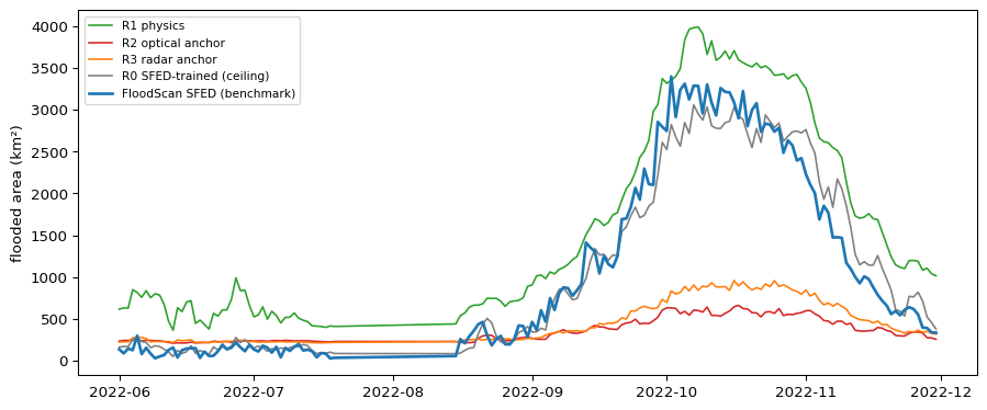
The physics route wins, and not narrowly: r = 0.84 against SFED and 99% of
its peak area, from a literature constant and the pixel's own history. The
anchor routes fail for a structural reason worth remembering: 2022 flooded
beyond anything in their anchors' experience, so amplitudes calibrated to
Landsat history or three radar snapshots cap out far too low. You cannot
anchor an extreme to a record that never contained one.
R1's one visible flaw is a dry-season floor: a few hundred km² of low-level
"flood" in June-August where SFED reports almost none, from soil moisture
and seasonal wetness leaking into the signal. FloodScan's Users Guide
documents the identical problem and its fix, a "minimum detectable flooded
fraction (MDFF) threshold" applied to filter "low level flooded fraction
noise" (v05R01, §1.2). Applying the same idea (zero out fractions below
0.10) cuts our June floor to SFED's level while keeping r = 0.83 and 86% of
peak area. Independently rediscovering the need for their threshold is about
as strong a confirmation of the shared physics as one event can give.
## Test 3: allocation — the 83 m maps
The remaining stage is spatial. The historical water map is the JRC Global
Surface Water dataset (free, ~30 m, fetched here by reading just the needed
window over HTTP). This is the same dataset AER names as an ingredient of
FloodScan's downscaling database; their version also folds in topography and
hydrology layers, so our single-ingredient version is a floor on what the
technique can do, not a replica. Inside each 10 km pixel we sort the small
cells from most to least water-prone, exclude cells that are water
year-round (lakes, the river channel itself), and mark cells as flooded from
the top of the list until the pixel's estimated share is reached.
One method note before the maps: the allocation experiments below were run
with the **R0 fraction as the GFDS-side input** (they predate the R1
results; re-running them on R1 is listed in the next steps). The scripts:
```{python}
#| eval: false
#| code-summary: "experiments/gfds_downscaling_poc/02_build_prior.py"
{{< include ../experiments/gfds_downscaling_poc/02_build_prior.py >}}
```
```{python}
#| eval: false
#| code-summary: "experiments/gfds_downscaling_poc/04_downscale_validate.py"
{{< include ../experiments/gfds_downscaling_poc/04_downscale_validate.py >}}
```
### Head to head: downscaled GFDS vs downscaled FloodScan
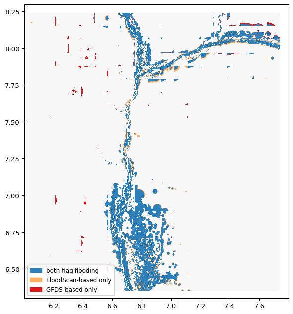
Test 1 compared the two products at the calibration stage, on the 10 km
grid. This figure is the next stage of the same story: the same two 10 km
fractions, now pushed through the identical allocation, compared as 83 m
maps over the confluence for the October peak.
```{python}
#| fig-cap: "CALIBRATION + ALLOCATION, ~83 m. The same two 10 km fractions from Test 1 after downscaling, Niger-Benue confluence, 6-13 Oct 2022. Blue = both flag flooding, orange = only the FloodScan-based map, red = only the GFDS-based map."
#| fig-height: 8
from matplotlib.colors import ListedColormap
from matplotlib.patches import Patch

z = np.load(POC / "downscale_maps.npz")
gfm_wet, ds_gfds, ds_sfed, ctrl, dom = (z[k] for k in
                                        ("gfm_wet", "ds_gfds", "ds_sfed", "ctrl", "dom"))
ext = [z["x"].min(), z["x"].max(), z["y"].min(), z["y"].max()]

cat = np.zeros(ds_gfds.shape, dtype=float)
cat[ds_sfed & ds_gfds] = 1
cat[ds_sfed & ~ds_gfds] = 2
cat[~ds_sfed & ds_gfds] = 3
cmap = ListedColormap(["#f7f7f7", "#2c7fb8", "#fdae61", "#d7191c"])
fig, ax = plt.subplots(figsize=(8, 8))
ax.imshow(np.where(dom, cat, np.nan), extent=ext, cmap=cmap,
          vmin=-0.5, vmax=3.5, interpolation="none")
ax.set_aspect("equal")
ax.legend(handles=[
    Patch(color="#2c7fb8", label="both flag flooding"),
    Patch(color="#fdae61", label="FloodScan-based only"),
    Patch(color="#d7191c", label="GFDS-based only")],
    loc="lower left", fontsize=9, framealpha=0.9)
plt.show()

both_n = int((ds_gfds & ds_sfed & dom).sum())
either_n = int(((ds_gfds | ds_sfed) & dom).sum())
a_g = int((ds_gfds & dom).sum()) * 0.0835**2
a_s = int((ds_sfed & dom).sum()) * 0.0835**2
print(f"flooded area: GFDS-based {a_g:,.0f} km2 | FloodScan-based {a_s:,.0f} km2 "
      f"(ratio {a_g/a_s:.2f})")
print(f"overlap: {both_n/either_n:.0%} of all cells flagged by either map "
      "are flagged by both")
```
The two maps flag nearly the same total area and mostly the same cells; the
disagreements sit at pixel edges where the two 10 km inputs put slightly
different amounts into neighbouring pixels. Through an identical recipe, the
free input substitutes for the licensed one with little visible cost.
Whether either map is *right* is a separate question, which needs a
reference from outside the microwave family.
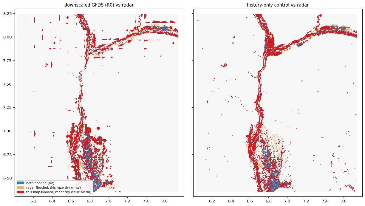
### An outside check: radar, and a control with no satellite input
For that we borrow this project's GFM data: Sentinel-1 radar flood extent
for the same dates. Radar is a different product with a different overpass
cadence, so disagreement with the daily microwave products is expected and
does not crown a winner; its job here is only to arbitrate one narrow
question. Alongside the two downscaled maps we score a third: the
**history-only control** defined in the methods section, same total flooded
area, no 2022 satellite input. If the satellite-based maps cannot beat the
control against the radar, the fine detail is coming from the historical
map, not from either satellite product.
```{python}
#| fig-cap: "Niger-Benue confluence, 6-13 Oct 2022, ~83 m. Each panel compares one map against the radar: blue = both flag flooding, orange = radar flags flooding the map missed, red = the map flags flooding the radar did not see. Left: downscaled GFDS (R0 fraction). Right: the history-only control. GFDS converts orange to blue across the wide flooding south of the confluence, at the cost of red false alarms in rectangular blocks at pixel edges."
#| fig-height: 7
def agreement(pred):
    cat = np.zeros(pred.shape, dtype=float)          # 0: dry in both
    cat[gfm_wet & pred] = 1                           # both wet
    cat[gfm_wet & ~pred] = 2                          # radar only
    cat[~gfm_wet & pred] = 3                          # map only
    return np.where(dom, cat, np.nan)

cmap = ListedColormap(["#f7f7f7", "#2c7fb8", "#fdae61", "#d7191c"])
fig, axes = plt.subplots(1, 2, figsize=(13, 7), sharex=True, sharey=True)
for ax, pred, title in [(axes[0], ds_gfds, "downscaled GFDS (R0) vs radar"),
                        (axes[1], ctrl, "history-only control vs radar")]:
    ax.imshow(agreement(pred), extent=ext, cmap=cmap, vmin=-0.5, vmax=3.5,
              interpolation="none")
    ax.set_title(title, fontsize=11)
    ax.set_aspect("equal")
axes[0].legend(handles=[
    Patch(color="#2c7fb8", label="both flooded (hit)"),
    Patch(color="#fdae61", label="radar flooded, this map dry (miss)"),
    Patch(color="#d7191c", label="this map flooded, radar dry (false alarm)")],
    loc="lower left", fontsize=8, framealpha=0.9)
plt.tight_layout()
plt.show()
```
```{python}
#| code-summary: "scores at 83 m"
def score(pred):
    h = int((pred & gfm_wet & dom).sum())
    f = int((pred & ~gfm_wet & dom).sum())
    m = int((~pred & gfm_wet & dom).sum())
    return {"POD/Recall": round(h / (h + m), 3),
            "FAR (1−Precision)": round(f / (h + f), 3),
            "CSI/IoU": round(h / (h + m + f), 3)}

zr1 = np.load(POC / "r1_downscaled.npz")  # from script 07
pd.DataFrame({"downscaled GFDS (R0, SFED-trained)": score(ds_gfds),
              "downscaled GFDS (R1 physics, independent)": score(zr1["ds_r1"]),
              "downscaled GFDS (R1 + MDFF 0.10)": score(zr1["ds_r1m"]),
              "downscaled SFED (licensed)": score(ds_sfed),
              "history-only control": score(ctrl)}).T
```
POD is the share of radar-flooded cells the map caught, FAR the share of
the map's flooded cells the radar contradicts, CSI the overall overlap.
Two results at full 83 m detail are uncomfortable and worth stating plainly.
First, **the history-only control ties the maps that used satellite data**.
Second, the fully independent chain (R1 physics fraction through the same
allocation) currently scores *below* all of them: its peak-window amplitude
runs high, painting roughly half again more area than the R0 version, and
the radar punishes the over-spread as false alarms. Independence is
demonstrated at 10 km; at 83 m it still needs amplitude tuning. The
figure shows a visible difference, yet cell by cell the gains on the
floodplain are cancelled by the block-edge false alarms. Also notable: the
free GFDS input scores within a whisker of the licensed FloodScan input. One
fairness note about the reference: radar under-detects water beneath
vegetation, and we compare three radar snapshots against continuous microwave
coverage, so part of every map's "red" reflects the reference's blind spots
rather than the map's errors.
### Where it really flooded: beyond the historical envelope
A fair objection to everything above: cells with Landsat water history are
easy, the fill paints them first, so scores there flatter every map. The
telling stratum is the cells *outside* the historical envelope, where water
appeared in places the 1984-2021 record never saw it. Detection there cannot
come from water history.
```{python}
#| code-summary: "stratify the radar comparison by the historical water envelope"
prior = np.load(POC / "gsw_prior_aoi.npz")
occ = prior["occ"]
inside = dom & (occ > 0)
outside = dom & (occ == 0)
wet_in = int((gfm_wet & inside).sum())
wet_out = int((gfm_wet & outside).sum())
print(f"radar-flooded cells with water history: {wet_in:,} | without: {wet_out:,} "
      f"({wet_out/(wet_in+wet_out):.0%} of the flood was outside the envelope)")

rows = {}
for name, pred in [("R0 (SFED-trained)", ds_gfds),
                   ("R1 physics", zr1["ds_r1"]),
                   ("SFED (licensed)", ds_sfed),
                   ("history-only control", ctrl)]:
    hi = int((pred & gfm_wet & inside).sum()); mi = int((~pred & gfm_wet & inside).sum())
    ho = int((pred & gfm_wet & outside).sum()); mo = int((~pred & gfm_wet & outside).sum())
    fo = int((pred & ~gfm_wet & outside).sum())
    rows[name] = {"POD/Recall inside": round(hi/(hi+mi), 2),
                  "POD/Recall outside": round(ho/(ho+mo), 2),
                  "FAR outside": round(fo/(ho+fo), 2),
                  "CSI/IoU outside": round(ho/(ho+mo+fo), 3)}
pd.DataFrame(rows).T
```
Three things fall out. First, the headline: **85% of this flood happened in
cells with no Landsat water history at all**. A flood mask built from
historical water alone would have missed most of the event; that single
number is the case for satellite monitoring of extremes. Second, inside the
envelope everyone scores near-perfect detection, confirming that stratum
tells you nothing. Third, outside the envelope the satellite-informed maps
do detect more (licensed SFED reaches 0.64 recall, R0 0.57, against 0.53
for the control) but no more precisely, so the overlap scores still tie.
One design honesty note explains why the control stays competitive even
here: its tie-break ranks cells by distance to historical water, and since
rivers flood outward, proximity geometry alone predicts much of even the
novel flooding. Strictly, the control is "history plus geometry", and at
83 m that combination remains hard for a 10 km satellite signal to beat.
### Zooming out: where the satellite earns its keep
If the fine detail is mostly the historical map, the satellite has to prove
itself at coarser zoom. We blur all the maps to a series of coarser grids
and check how well each tracks the radar:
```{python}
#| code-summary: "agreement with radar (correlation) at increasing blur"
def block_reduce(a, k, m):
    ny, nx = a.shape
    ny2, nx2 = ny // k * k, nx // k * k
    aa = np.where(m, a, np.nan)[:ny2, :nx2].reshape(ny2 // k, k, nx2 // k, k)
    with np.errstate(invalid="ignore"):
        return np.nanmean(np.nanmean(aa, axis=3), axis=1)

rows = []
for k, label in [(1, "83 m"), (6, "0.5 km"), (12, "1 km"), (36, "3 km"), (72, "6 km")]:
    g = block_reduce(gfm_wet.astype(float), k, dom)
    vs = block_reduce(dom.astype(float), k, np.ones_like(dom, bool))
    mm = np.isfinite(g) & (vs > 0.5)
    row = {"scale": label}
    for name, pred in [("GFDS (R0)", ds_gfds), ("SFED", ds_sfed),
                       ("history-only control", ctrl)]:
        p = block_reduce(pred.astype(float), k, dom)
        ok = mm & np.isfinite(p)
        row[name] = round(float(np.corrcoef(p[ok], g[ok])[0, 1]), 3)
    rows.append(row)
pd.DataFrame(rows).set_index("scale")
```
Now the picture is clean. At 83 m all three maps agree with the radar equally
(and equally poorly). At coarser evaluation grids, the two maps built from
2022 satellite data pull ahead of the control by a clear margin from 3 km
out. And at every level, free GFDS sits within a hair of licensed
FloodScan.
## What this settles
1. **The useful product is the calibrated 10 km fraction, not the 83 m map.**
It gives GFDS physical units, comparable across pixels and summable into
areas and exposure estimates. That is what admin-level monitoring
consumes, and it costs nothing.
2. **The 83 m map is an allocation of the coarse estimate, not an
observation.** It is a reasonable way to decide which communities inside a
pixel to count when overlaying population, but it must never be read as
observed flood extent.
3. **Both open-source questions survive their first test.** Reproduction:
the R0 lookup matches the licensed product at 10 km, and through the
identical allocation the two 83 m maps overlap on 84% of flagged cells
with a 0.91 area ratio. Independence: the R1 physics calibration needs no
licensed data at all and reaches r = 0.84 and 99% of peak area against
the licensed product.
The path from "free copy" to "maybe better" now has concrete work items:
refine R1 (per-pixel emissivity contrast, a seasonal dry reference instead
of one quantile, a tuned minimum-detectable threshold — the allocation test
above shows its amplitude runs hot at the peak, so this tuning is what
stands between "independent at 10 km" and "independent end to end"), train
on the 28-year free archive rather than one season, add terrain to the
historical map, and replicate on a second basin. The free input's finer working resolution (~10 km vs ~22 km)
is the standing structural advantage.