---
jupyter: ds-flood-gfm
---
## Cameroon Flood Snapshots
Analysis of October & November 2024 flooding events in Cameroon using GFM (Global Flood Monitoring) satellite data. We compare GFM-derived affected population estimates against FloodScan and CEMS reference data.
```{python}
import pystac_client
import stackstac
import matplotlib.pyplot as plt
from matplotlib.colors import ListedColormap, BoundaryNorm
import numpy as np
import geopandas as gpd
from fsspec.implementations.http import HTTPFileSystem
from ds_flood_gfm.geo_utils import load_adm0_lowres
import time
import pandas as pd

import ocha_stratus as stratus
from datetime import datetime, timedelta
from exactextract import exact_extract
# Configure matplotlib for better display
%matplotlib inline
plt.rcParams['figure.dpi'] = 100
```
```{python}
# Analysis configuration
notebook_config = {
    'combined_range': {
        'start': '2024-10-14',
        'end': '2024-11-30'
    },
    'october': {
        'name': 'October 2024 Floods',
        'start': '2024-10-14',
        'end': '2024-10-30',
        'snapshot_dates': ['2024-10-18', '2024-10-25'],
        'reference_date': '2024-10-18'
    },
    'november': {
        'name': 'November 2024 Floods',
        'start': '2024-11-13',
        'end': '2024-11-30',
        'snapshot_dates': ['2024-11-23', '2024-11-28'],
        'reference_date': '2024-11-18'
    }
}
```
## Area of Interest
Analysis focuses on Admin 1 region CM004 in Cameroon, with three custom AOI polygons defined by Copernicus Emergency Management Service (EMSR772 & EMSR779).
```{python}
GLOBAL_ADM1 = (
    "https://data.fieldmaps.io/edge-matched/humanitarian/intl/adm1_polygons.parquet"
)
ISO3 = "CMR"
filesystem = HTTPFileSystem()
filters = [("iso_3", "=", ISO3)]
gdf = gpd.read_parquet(GLOBAL_ADM1, filesystem=filesystem, filters=filters)
gdf_aoi = gdf[gdf.adm1_src == "CM004"]
bbox = gdf_aoi.total_bounds
```
```{python}
gdf_world_adm0 = load_adm0_lowres()
gdf_subset_admo = gdf_world_adm0[gdf_world_adm0.name == "Cameroon"]
```
```{python}
# load specific aoi used by copernicus
laoi = []
for aoi_num in range(1, 4):
    _blob_name = f"ds-cmr-flooding-support/raw/copernicus/EMSR772_AOI{aoi_num:02d}_DEL_PRODUCT_v1.zip"
    _shapefile = f"EMSR772_AOI{aoi_num:02d}_DEL_PRODUCT_areaOfInterestA_v1.shp"
    aoi_gdf = stratus.load_shp_from_blob(
        blob_name=_blob_name, shapefile=_shapefile, container_name="projects"
    )
    laoi.append(aoi_gdf)

gdf_aoi_copernicus = gpd.pd.concat(laoi, ignore_index=True)
```
## STAC Query
Query GFM flood extent data from EODC STAC API for the combined date range (Oct 14 - Nov 30, 2024).
```{python}
# | cache: true
# | cache-comments: "Cache STAC search results - change dates to invalidate"
stac_api = "https://stac.eodc.eu/api/v1"
client = pystac_client.Client.open(stac_api)

# Query for combined date range covering both October and November events
start_date = notebook_config['combined_range']['start']
end_date = notebook_config['combined_range']['end']

# Step 2: Search for GFM items
datetime_range = f"{start_date}/{end_date}"
search = client.search(
    collections=["GFM"],
    bbox=gdf_aoi.total_bounds,
    datetime=datetime_range,
)

item_collection = search.item_collection()
```
```{python}
#| cache: true
#| cache-lazy: true
stack = stackstac.stack(item_collection, epsg=4326)
```
## Pre-Processing
### GFM Data (STAC) Lazy
Extract flood extent band and create daily composites by taking the maximum flood value per day across overlapping tiles.
```{python}
# | cache: true
# | cache-lazy: true
stack_flood = stack.sel(band="ensemble_flood_extent")

stack_flood_clipped = stack_flood.sel(
x=slice(bbox[0], bbox[2]), y=slice(bbox[3], bbox[1])  # y is reversealri
)

# Group by day and take the maximum flood value for each day
# Use groupby instead of resample to only get days that actually have data
stack_flood_max = stack_flood_clipped.groupby("time.date").max()

# Rename the dimension back to 'time' and convert to datetime
stack_flood_max = stack_flood_max.rename({"date": "time"})
stack_flood_max["time"] = stack_flood_max.time.astype("datetime64[ns]")
```
Split the combined dataset into October and November events before applying forward-fill. This is more efficient since forward-fill is a sequential operation that processes all timesteps.
```{python}
# Split into individual events using config dates (before ffill for performance)
oct_stack_flood_max = stack_flood_max.sel(
    time=slice(notebook_config['october']['start'], notebook_config['october']['end'])
)
nov_stack_flood_max = stack_flood_max.sel(
    time=slice(notebook_config['november']['start'], notebook_config['november']['end'])
)

# Apply forward-fill separately to each event (much more efficient)
oct_ic_latest = oct_stack_flood_max.ffill(dim="time")
nov_ic_latest = nov_stack_flood_max.ffill(dim="time")
```
```{python}
#| eval: false
#| echo: false
def print_mb(da):
print(f"Size in memory: {da.nbytes / 1024**2:.1f} MB")
```
### Population Data (GHSL)
Load GHSL population data to overlay. Here we are using the estimated 2025 pop produced in 2023.
- We load it just for the AOI bbox, then clip it down further.
```{python}
blob_name = "ghsl/pop/GHS_POP_E2025_GLOBE_R2023A_4326_3ss_V1_0.tif"
da_global = stratus.open_blob_cog(blob_name, container_name="raster").squeeze(drop=True)

# Ensure the global data has the correct CRS
# da_global = da_global.rio.write_crs("EPSG:4326")
da_global.rio.crs

# clip to box (need to do this first, otherwise Python crashes on normal .rio.clip)
min_x, min_y, max_x, max_y = gdf_aoi.total_bounds
da_clip_box = da_global.rio.clip_box(minx=min_x, miny=min_y, maxx=max_x, maxy=max_y)

# clip to admin and preserve CRS
da_clip = da_clip_box.rio.clip(gdf_aoi.geometry)
da_clip = da_clip.rio.write_crs("EPSG:4326")
da_clip = da_clip.where(da_clip != da_clip.rio.nodata)
```
```{python}
#| eval: false
#| echo: false
# Load local GHSL population data
import rioxarray as rxr
# Load the local GeoTIFF file
da_local = rxr.open_rasterio(
"data/ghsl_e2020/GHS_POP_E2020_GLOBE_R2023A_4326_3ss_V1_0_R8_C20.tif"
).squeeze(drop=True)
# Ensure the local data has the correct CRS
da_local = da_local.rio.write_crs("EPSG:4326")
# clip to box (need to do this first, otherwise Python crashes on normal .rio.clip)
min_x, min_y, max_x, max_y = gdf_aoi.total_bounds
da_local_clip_box = da_local.rio.clip_box(
minx=min_x, miny=min_y, maxx=max_x, maxy=max_y
)
# clip to admin and preserve CRS
da_local_clip = da_local_clip_box.rio.clip(gdf_aoi.geometry)
da_local_clip = da_local_clip.rio.write_crs("EPSG:4326")
# Create a map to visualize overlap between local population data and AOI
fig, ax = plt.subplots(1, 1, figsize=(12, 8))
# Check coordinate ranges
print(f"da_local_clip bounds: {da_local_clip.rio.bounds()}")
print(f"gdf_aoi bounds: {gdf_aoi.total_bounds}")
print(f"da_local_clip CRS: {da_local_clip.rio.crs}")
print(f"gdf_aoi CRS: {gdf_aoi.crs}")
# Plot the local population data with manual extent setting
im = da_local_clip.plot(ax=ax, cmap="YlOrRd", vmin=0, vmax=200, add_colorbar=False)
# Add colorbar
cbar = plt.colorbar(im, ax=ax, label="Population Count")
# Add AOI boundary
gdf_aoi.boundary.plot(ax=ax, color="red", linewidth=3, alpha=1.0)
# Set axis limits to the AOI bounds to ensure visibility
ax.set_xlim(gdf_aoi.total_bounds[0], gdf_aoi.total_bounds[2])
ax.set_ylim(gdf_aoi.total_bounds[1], gdf_aoi.total_bounds[3])
# Set title and labels
ax.set_title(
"Local Population Data 2020 - Overlap with AOI", fontsize=12, fontweight="bold"
)
ax.set_xlabel("Longitude")
ax.set_ylabel("Latitude")
plt.tight_layout()
plt.show()
```
```{python}
# | eval: false
# | echo: false
print(f"da_clip fill value: {da_clip.rio.nodata}")
print(f"da_clip has NaNs: {da_clip.isnull().any().values}")
print(f"da_clip min (should be 0): {da_clip.min().values}")
da_clip = da_local_clip
# Or more robust - use the nodata value
# Verify
print(
f"da_clip min after masking: {da_clip.min().values}"
) # Should be 0 or small positive
print(f"da_clip has NaNs: {da_clip.isnull().any().values}") # Should be True
```
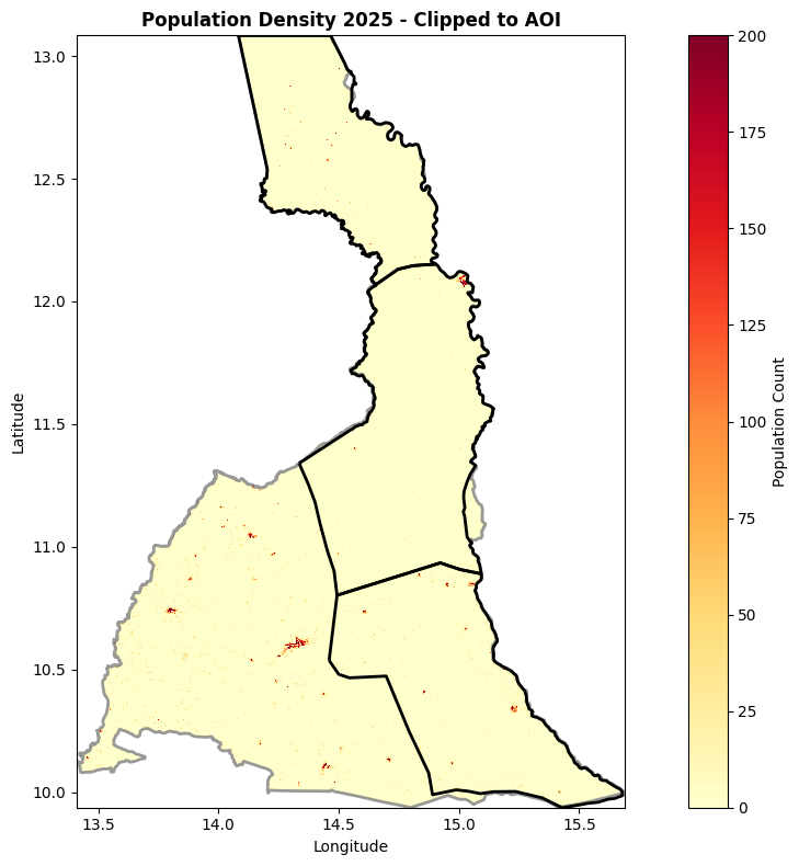
Here we show the GHSL population raster for the admin 1 of interest (grey outline) and the specific custom AOI's from CEMS (black outline).
```{python}
# Create a map of the clipped population data
fig, ax = plt.subplots(1, 1, figsize=(12, 8))

# Plot the population data
im = da_clip.plot(
    ax=ax,
    cmap='YlOrRd',
    vmin=0,
    vmax=200,
    add_colorbar=False
)

# Add colorbar
cbar = plt.colorbar(im, ax=ax, label='Population Count')

# Add admin boundary in grey
gdf_aoi.boundary.plot(ax=ax, color='grey', linewidth=2, alpha=0.8)

# Add Copernicus AOI boundaries in black
gdf_aoi_copernicus.boundary.plot(ax=ax, color='black', linewidth=2, alpha=1.0)

# Set title and labels
ax.set_title('Population Density 2025 - Clipped to AOI', fontsize=12, fontweight='bold')
ax.set_xlabel('Longitude')
ax.set_ylabel('Latitude')

plt.tight_layout()
plt.show()
```
```{python}
#| eval: false
#| echo: false
print(f"da_clip dtype: {da_clip.dtype}")
print(f"da_clip nodata: {da_clip.rio.nodata}")
print(f"da_clip min: {da_clip.min().values}")
print(f"da_clip max: {da_clip.max().values}")
print(f"da_clip sum: {da_clip.sum(skipna=True).values:,.0f}")
print(f"da_clip has NaN: {da_clip.isnull().any().values}")
print(f"da_clip has negative: {(da_clip < 0).any().values}")
```
## Overlay Flood Extent & Population Data
Here we follow the GFM methodology as closely as possible. We need to get the data on comparable grids:
- We take the 100m population data and resample it to the 20m flood data and rescale the population numbers to reflect this.
- We then run zonal statistics (using `exact_extract`)
```{python}
def gfm_exact_workflow_zonal(flood_20m, population_100m, gdf_zones, zone_id_col=None):
    """
    Calculate affected population using GFM methodology with zonal statistics.

    Parameters
    ----------
    flood_20m : xr.DataArray
        Binary flood mask at 20m resolution (0 or 1)
    population_100m : xr.DataArray
        Population density at 100m resolution
    gdf_zones : gpd.GeoDataFrame
        Polygons for zonal statistics (e.g., multiple admin areas)
    zone_id_col : str, optional
        Column name to use as zone identifier

    Returns
    -------
    pd.DataFrame
        Results with affected_population per zone
    """

    print("=" * 80)
    print("GFM Exact Workflow with Zonal Statistics (exactextract)")
    print("=" * 80)

    print(f"\nNumber of zones: {len(gdf_zones)}")

    # Ensure CRS match
    if gdf_zones.crs != flood_20m.rio.crs:
        print(f"Reprojecting zones from {gdf_zones.crs} to {flood_20m.rio.crs}")
        gdf_zones = gdf_zones.to_crs(flood_20m.rio.crs)

    # Clean population nodata
    if population_100m.rio.nodata is not None:
        print(f"Clearing nodata metadata (was: {population_100m.rio.nodata})")
        population_100m = population_100m.rio.write_nodata(None)

    # Resample population to 20m
    print("Upsampling population from 100m to 20m...")
    population_20m = population_100m.rio.reproject_match(
        flood_20m,
        resampling=0  # nearest neighbor
    )

    # Adjust for pixel area (divide by 25)
    print("Adjusting population density for resolution change...")
    pixel_area_ratio = (100 / 20) ** 2  # = 25
    population_20m_adjusted = population_20m / pixel_area_ratio

    print(f"  Population adjustment factor: {pixel_area_ratio}")
    print(f"  Original sum: {population_100m.sum(skipna=True).values:,.0f}")
    print(f"  After adjustment: {population_20m_adjusted.sum(skipna=True).values:,.0f}")

    # Calculate affected population
    print("Calculating affected population at 20m resolution...")
    affected_pop_20m = flood_20m * population_20m_adjusted

    # Zonal statistics using exactextract
    print(f"Computing zonal statistics for {len(gdf_zones)} zones...")

    # Prepare zone identifier
    if zone_id_col and zone_id_col in gdf_zones.columns:
        zone_ids = gdf_zones[zone_id_col].tolist()
    else:
        zone_ids = gdf_zones.index.tolist()

    # Extract zonal sums for affected population
    results = exact_extract(
        affected_pop_20m,
        gdf_zones,
        'sum',
        output='pandas'
    )

    # Extract flood extent statistics
    flood_results = exact_extract(
        flood_20m,
        gdf_zones,
        ['sum', 'count'],
        output='pandas'
    )

    # Combine results
    results_df = pd.DataFrame({
        'zone_id': zone_ids,
        'affected_population': results['sum'].values,
        'flooded_pixels': flood_results['sum'].values,
        'total_pixels': flood_results['count'].values,
    })

    # Calculate flooded area
    pixel_area_m2 = 20 * 20  # 20m resolution
    results_df['flooded_area_m2'] = results_df['flooded_pixels'] * pixel_area_m2
    results_df['flooded_area_km2'] = results_df['flooded_area_m2'] / 1_000_000

    # Add zone names if available
    if zone_id_col and zone_id_col in gdf_zones.columns:
        results_df['zone_name'] = gdf_zones[zone_id_col].values

    # Clean up values
    results_df['affected_population'] = results_df['affected_population'].fillna(0).astype(int)
    results_df['flooded_pixels'] = results_df['flooded_pixels'].fillna(0).astype(int)

    print("\n" + "=" * 80)
    print("RESULTS BY ZONE")
    print("=" * 80)
    print(results_df.to_string(index=False))

    return results_df
```
```{python}
def map_flood_extent_snapshots(flood_data_computed, snapshot_dates, gdf_boundaries, event_name):
    """
    Create side-by-side flood extent maps for snapshot dates.

    Parameters
    ----------
    flood_data_computed : xr.DataArray
        Computed flood data array (already filtered and computed)
    snapshot_dates : list
        List of snapshot dates being visualized
    gdf_boundaries : gpd.GeoDataFrame
        Boundaries to overlay on maps
    event_name : str
        Event name for plot context

    Returns
    -------
    None
        Displays matplotlib figure
    """
    # Define colors for flood data visualization
    colors = ["lightgrey", "darkblue", "white"]  # 0=no flood, 1=flood, 255=nodata
    cmap = ListedColormap(colors)
    bounds = [0, 0.5, 1.5, 255.5]
    norm = BoundaryNorm(bounds, cmap.N)

    fig, (ax1, ax2) = plt.subplots(1, 2, figsize=(20, 8))

    # Process each time step
    for i, ax in enumerate([ax1, ax2]):
        time_step = flood_data_computed.isel(time=i)
        date_str = str(time_step.time.values)[:10]

        # Process data (handle NaN and downsample for visualization)
        data_clean = np.where(np.isnan(time_step), 255, time_step)
        data_clean = data_clean[::4, ::4]  # Downsample for speed

        # Get extent from the xarray data
        bounds_extent = time_step.rio.bounds()
        extent = [bounds_extent[0], bounds_extent[2], bounds_extent[1], bounds_extent[3]]

        # Plot the flood data
        im = ax.imshow(
            data_clean,
            cmap=cmap,
            norm=norm,
            interpolation="nearest",
            origin="upper",
            extent=extent,
        )

        # Overlay boundaries
        gdf_boundaries.boundary.plot(ax=ax, color='red', linewidth=3, alpha=0.8)

        # Set title and labels
        ax.set_title(f'{event_name}\nFlood Extent - {date_str}',
                    fontsize=12, fontweight='bold')
        ax.set_xlabel('Longitude')
        ax.set_ylabel('Latitude')

    plt.tight_layout()
    plt.show()
```
```{python}
def create_comparison_barplot(gfm_results, other_systems_data, event_name,
                              systems=['CEMS', 'FloodScan', 'GFM (STAC)']):
    """
    Create comparison bar plot of affected population across systems.

    Parameters
    ----------
    gfm_results : pd.DataFrame
        GFM zonal statistics results with columns: zone_id, affected_population
    other_systems_data : dict
        Dict of system data, e.g., {'FloodScan': {'AOI 1': 7580, ...}, 'CEMS': {...}}
    event_name : str
        Event name for plot title
    systems : list
        List of systems to include in plot (e.g., ['CEMS', 'GFM (STAC)'])

    Returns
    -------
    None
        Displays matplotlib figure and prints comparison stats
    """
    # Convert other systems data to DataFrame
    comparison_data = []
    for system, values in other_systems_data.items():
        for aoi, pop in values.items():
            comparison_data.append({
                'AOI': aoi,
                'System': system,
                'affected_population': pop
            })

    df_other_systems = pd.DataFrame(comparison_data)

    # Prepare GFM data
    gfm_comparison = gfm_results[['zone_id', 'affected_population']].copy()
    gfm_comparison['System'] = 'GFM (STAC)'

    # Map zone_id to standard AOI format
    zone_id_to_aoi = {}
    for idx, zone_id in enumerate(gfm_comparison['zone_id']):
        if isinstance(zone_id, (int, np.integer)):
            zone_id_to_aoi[zone_id] = f"AOI {zone_id + 1}"
        elif 'AOI' in str(zone_id).upper():
            import re
            match = re.search(r'AOI(\d+)', str(zone_id), re.IGNORECASE)
            if match:
                aoi_num = int(match.group(1))
                zone_id_to_aoi[zone_id] = f"AOI {aoi_num}"
            else:
                zone_id_to_aoi[zone_id] = f"AOI {idx + 1}"
        else:
            zone_id_to_aoi[zone_id] = f"AOI {idx + 1}"

    gfm_comparison['AOI'] = gfm_comparison['zone_id'].map(zone_id_to_aoi)
    gfm_comparison = gfm_comparison[['AOI', 'System', 'affected_population']]

    # Combine all data
    df_combined = pd.concat([df_other_systems, gfm_comparison], ignore_index=True)

    # Filter to requested systems
    df_combined = df_combined[df_combined['System'].isin(systems)]

    # Display comparison table
    print("\n" + "=" * 80)
    print(f"AFFECTED POPULATION COMPARISON - {event_name}")
    print("=" * 80)
    print(df_combined.pivot(index='AOI', columns='System', values='affected_population'))

    # Create comparison barplot
    fig, ax = plt.subplots(figsize=(12, 6))

    # Get unique AOIs and systems
    aois = sorted(df_combined['AOI'].unique())
    systems_plot = [s for s in systems if s in df_combined['System'].values]

    # Set up bar positions
    x = np.arange(len(aois))
    width = 0.8 / len(systems_plot)  # Adjust width based on number of systems

    # Define consistent colors
    color_map = {
        'GFM (STAC)': '#3cb371',      # Minty green
        'FloodScan': '#ff6347',        # Tomato red
        'CEMS': '#0f52ba'              # Sapphire blue
    }

    # Plot bars for each system
    for i, system in enumerate(systems_plot):
        system_data = df_combined[df_combined['System'] == system]
        values = [system_data[system_data['AOI'] == aoi]['affected_population'].values[0]
                  if len(system_data[system_data['AOI'] == aoi]) > 0 else 0
                  for aoi in aois]

        bars = ax.bar(x + i * width, values, width, label=system, color=color_map.get(system, 'gray'))

        # Add value labels on bars
        for bar, val in zip(bars, values):
            height = bar.get_height()
            ax.text(bar.get_x() + bar.get_width()/2., height,
                    f'{int(val):,}',
                    ha='center', va='bottom', fontsize=9)

    # Customize plot
    ax.set_xlabel('Area of Interest (AOI)', fontsize=12, fontweight='bold')
    ax.set_ylabel('Affected Population', fontsize=12, fontweight='bold')
    ax.set_title(f'Affected Population Comparison\n{event_name}', fontsize=14, fontweight='bold')
    ax.set_xticks(x + width * (len(systems_plot) - 1) / 2)
    ax.set_xticklabels(aois)
    ax.legend(title='System', loc='upper right', fontsize=11)
    ax.grid(axis='y', alpha=0.3, linestyle='--')

    # Format y-axis
    ax.yaxis.set_major_formatter(plt.FuncFormatter(lambda x, p: f'{int(x):,}'))

    plt.tight_layout()
    plt.show()

    # Print comparison ratios
    if 'GFM (STAC)' in systems_plot:
        print("\n" + "=" * 80)
        print("SYSTEM COMPARISON RATIOS (relative to GFM)")
        print("=" * 80)

        for aoi in aois:
            gfm_val = df_combined[(df_combined['AOI'] == aoi) & (df_combined['System'] == 'GFM (STAC)')]['affected_population'].values
            if len(gfm_val) > 0:
                gfm_val = gfm_val[0]
                print(f"\n{aoi}:")
                print(f"  GFM (baseline): {gfm_val:,}")

                for system in systems_plot:
                    if system != 'GFM (STAC)':
                        sys_val = df_combined[(df_combined['AOI'] == aoi) & (df_combined['System'] == system)]['affected_population'].values
                        if len(sys_val) > 0:
                            sys_val = sys_val[0]
                            ratio = sys_val / gfm_val if gfm_val > 0 else np.inf
                            print(f"  {system}: {sys_val:,} ({ratio:.2f}x GFM)")
```
## Resulting Flood Extents & Affected Population Zonal Stats
Calculate affected population for the November event using the forward-filled flood stack.
```{python}
#| cache: true
# Run zonal stats for November event using filled/forward-filled stack

flood_day_max = nov_stack_flood_max.sel(time=notebook_config['november']['snapshot_dates'])

flood_day_max_computed= flood_day_max.compute()
# Process each time step in flood_data_latest_computed
list_zonal = []

for i in range(len(flood_day_max_computed.time)):
    time_step = flood_day_max_computed.isel(time=i)
    date_str = str(time_step.time.values)[:10]
    print(f"\nProcessing {date_str}...")

    # Apply GFM threshold
    flood_day_max_binary = (time_step == 1).astype(int)
    flood_day_max_binary = flood_day_max_binary.rio.write_crs(time_step.rio.crs)

    # Run zonal analysis
    results_time = gfm_exact_workflow_zonal(
        flood_20m=flood_day_max_binary,
        population_100m=da_clip,
        gdf_zones=gdf_aoi_copernicus,
        zone_id_col='aoi_code'  # Adjust to match your column name
    )

    # Add date column to results
    results_time['date'] = date_str
    list_zonal.append(results_time)

    # Display results for this time step
    print(f"Total affected population for {date_str}: {results_time['affected_population'].sum():,}")

# Combine all results
day_max_zonal = pd.concat(list_zonal, ignore_index=True)
print(f"\nOverall results shape: {day_max_zonal.shape}")
day_max_zonal
```
```{python}
#| cache: true
# Zonal statistics using forward-filled composites (November event)

flood_data_latest = nov_ic_latest.sel(time=notebook_config['november']['snapshot_dates'])

flood_data_latest_computed = flood_data_latest.compute()

results_filled = []
for i in range(len(flood_data_latest_computed.time)):
    time_step = flood_data_latest_computed.isel(time=i)
    date_str = str(time_step.time.values)[:10]
    print(f"\nProcessing {date_str}...")

    # Apply GFM threshold
    flood_binary = (time_step == 1).astype(int)
    flood_binary = flood_binary.rio.write_crs(time_step.rio.crs)

    # Run zonal analysis
    results_time = gfm_exact_workflow_zonal(
        flood_20m=flood_binary,
        population_100m=da_clip,
        gdf_zones=gdf_aoi_copernicus,
        zone_id_col='aoi_code'  # Adjust to match your column name
    )

    # Add date column to results
    results_time['date'] = date_str
    results_filled.append(results_time)

    # Display results for this time step
    print(f"Total affected population for {date_str}: {results_time['affected_population'].sum():,}")

# Combine all results
nov_zonal_results = pd.concat(results_filled, ignore_index=True)

# Store the latest date result for comparison
nov_latest_img_zonal_date = nov_zonal_results[nov_zonal_results["date"] == notebook_config['november']['snapshot_dates'][0]]
```
### Flood Extent Visualizations
::: {.callout-tip collapse="true"}
## Why Latest-Day Composite is Beneficial
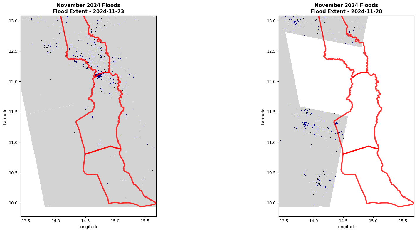
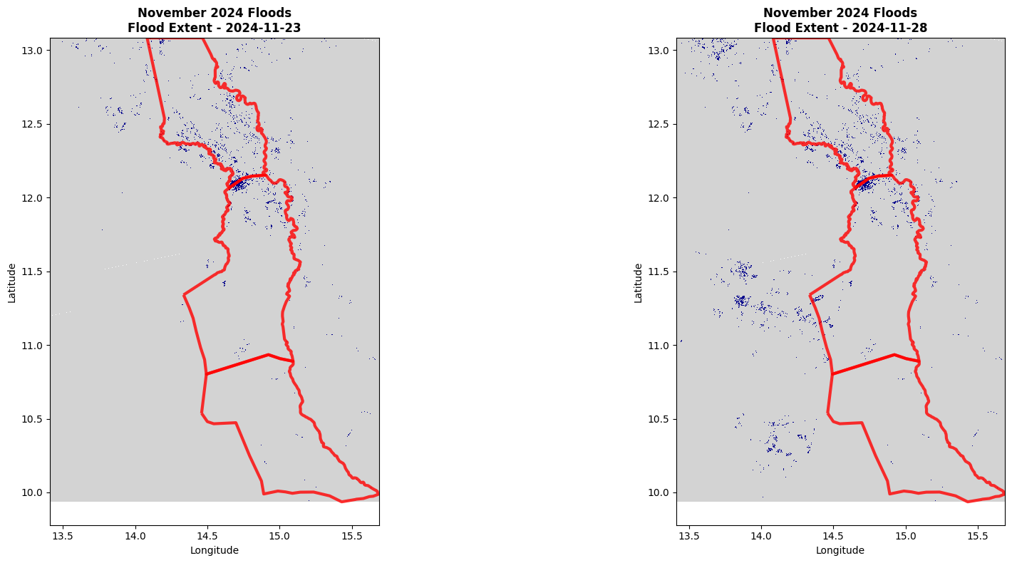
Individual satellite observations can have gaps largely due to overpass timing. Here we see the visualization. Here we see the flood extent of two single days around one of our flood event dates. In many use-cases we'd be interested in checking out a date and then we'd find the closest image with coverage. You can see the data gap present on Nov 28. If we ran zonal statistics on that image we'd end up with some confusing and misleading results. The `latest-image-composite` shown below will give us more useful results.
```{python}
#| cache: true
# Visualize flood extent for snapshot dates (individual observations only, no forward-fill)
map_flood_extent_snapshots(
    flood_data_computed=flood_day_max_computed,
    snapshot_dates=notebook_config['november']['snapshot_dates'],
    gdf_boundaries=gdf_aoi_copernicus,
    event_name=notebook_config['november']['name']
)
```
:::
```{python}
#| cache: true
# Visualize flood extent for snapshot dates (with forward-fill compositing)
map_flood_extent_snapshots(
    flood_data_computed=flood_data_latest_computed,
    snapshot_dates=notebook_config['november']['snapshot_dates'],
    gdf_boundaries=gdf_aoi_copernicus,
    event_name=notebook_config['november']['name']
)
```
### System Comparisons
```{python}
# Hardcoded November 2024 reference data from other systems
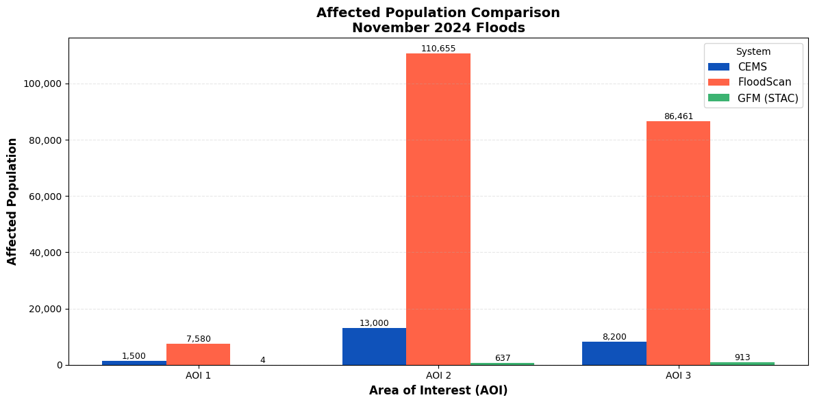
nov_other_systems_data = {
    'FloodScan': {
        'AOI 1': 7580,
        'AOI 2': 110655,
        'AOI 3': 86461
    },
    'CEMS': {
        'AOI 1': 1500,
        'AOI 2': 13000,
        'AOI 3': 8200
    }
}

# Create comparison plot with all three systems
create_comparison_barplot(
    gfm_results=nov_latest_img_zonal_date,
    other_systems_data=nov_other_systems_data,
    event_name=notebook_config['november']['name'],
    systems=['CEMS', 'FloodScan', 'GFM (STAC)']
)
```
## October 2024 Event Analysis
### Zonal Statistics
```{python}
#| cache: true
# Run zonal stats for October event using filled/forward-filled stack

oct_flood_data_latest = oct_ic_latest.sel(time=notebook_config['october']['snapshot_dates'])
oct_flood_data_latest_computed = oct_flood_data_latest.compute()

oct_results_filled = []
for i in range(len(oct_flood_data_latest_computed.time)):
    time_step = oct_flood_data_latest_computed.isel(time=i)
    date_str = str(time_step.time.values)[:10]
    print(f"\nProcessing {date_str}...")

    # Apply GFM threshold
    flood_binary = (time_step == 1).astype(int)
    flood_binary = flood_binary.rio.write_crs(time_step.rio.crs)

    # Run zonal analysis
    results_time = gfm_exact_workflow_zonal(
        flood_20m=flood_binary,
        population_100m=da_clip,
        gdf_zones=gdf_aoi_copernicus,
        zone_id_col='aoi_code'
    )

    # Add date column to results
    results_time['date'] = date_str
    oct_results_filled.append(results_time)

    # Display results for this time step
    print(f"Total affected population for {date_str}: {results_time['affected_population'].sum():,}")

# Combine all results
oct_zonal_results = pd.concat(oct_results_filled, ignore_index=True)

# Store the latest date result for comparison
oct_latest_img_zonal_date = oct_zonal_results[oct_zonal_results["date"] == notebook_config['october']['snapshot_dates'][0]]
```
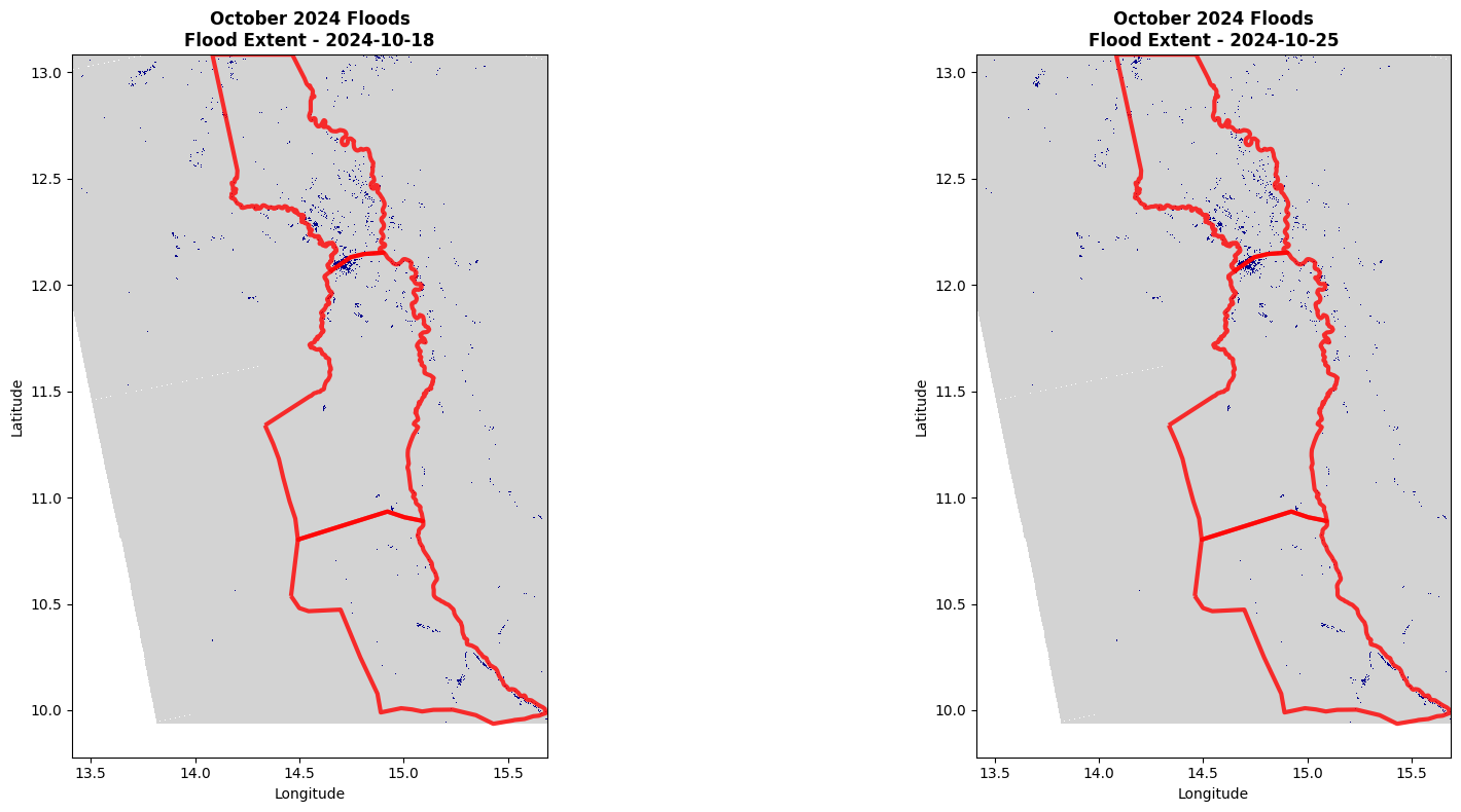
### Flood Extent Visualizations
```{python}
#| cache: true
# Visualize flood extent for October snapshot dates
map_flood_extent_snapshots(
    flood_data_computed=oct_flood_data_latest_computed,
    snapshot_dates=notebook_config['october']['snapshot_dates'],
    gdf_boundaries=gdf_aoi_copernicus,
    event_name=notebook_config['october']['name']
)
```
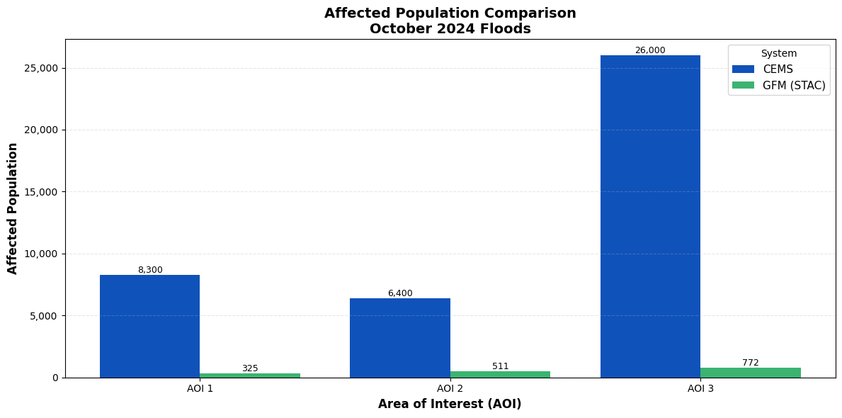
### System Comparisons
FloodScan data not available for October event.
```{python}
# Hardcoded October 2024 CEMS reference data
# TODO: Replace x, y, z with actual CEMS values for October
oct_other_systems_data = {
    'CEMS': {
        'AOI 1': 8300,
        'AOI 2': 6400,  # TODO: Add October CEMS value for AOI 2
        'AOI 3': 26000   # TODO: Add October CEMS value for AOI 3
    }
}

# Create comparison plot with CEMS and GFM only (no FloodScan)
create_comparison_barplot(
    gfm_results=oct_latest_img_zonal_date,
    other_systems_data=oct_other_systems_data,
    event_name=notebook_config['october']['name'],
    systems=['CEMS', 'GFM (STAC)']  # Only CEMS and GFM
)
```
## Appendix
```{python}
#| eval: false
#| echo: false
# All dates in ic_latest are actual observation dates (no filling needed)
# Create binary flood masks and calculate population impacts for each time step
ic_ready = stack_flood_max
population_impacts = []
dates = []
for i, time_step in enumerate(ic_ready.time):
print(f"\nProcessing date: {str(time_step.values)[:10]}")
try:
# Get flood data for this time step
flood_data = ic_ready.sel(time=time_step)
# Compute the data first to handle network errors
print(" Computing flood data from EODC...")
flood_data_computed = flood_data.compute()
# Create binary flood mask (1 = flooded, 0 = not flooded)
# Use GFM's official binary classification: exactly 1 = flood
# (ensemble requires 2 out of 3 algorithms to agree)
flood_binary = (flood_data_computed == 1).astype(int)
flood_binary = flood_binary.rio.write_crs(flood_data_computed.rio.crs)
# DEBUG: Check flood mask BEFORE resampling
print(
f" DEBUG - Unique values in flood_binary: {np.unique(flood_binary.values[~np.isnan(flood_binary.values)])}"
)
print(
f" DEBUG - Flooded cells BEFORE resample: {(flood_binary == 1).sum().values:,}"
)
# Resample flood data to match population grid resolution
# Population data is at higher resolution, so we need to align grids
# Use nearest neighbor (resampling=0) per GFM methodology
# https://rasterio.readthedocs.io/en/stable/api/rasterio.enums.html#rasterio.enums.Resampling
print(" Reprojecting to match population grid...")
flood_resampled = flood_binary.rio.reproject_match(
da_clip, resampling=0
) # 0 = Resampling.nearest (GFM spec)
except Exception as e:
print(f" ⚠️ ERROR: Failed to process {str(time_step.values)[:10]}: {e}")
print(f" Skipping this date...")
continue
# Calculate flooded population (multiply binary flood by population)
print(" Calculating affected population...")
# DEBUG: Check spatial extents and masking
print(f" DEBUG - flood_resampled extent: {flood_resampled.rio.bounds()}")
print(f" DEBUG - da_clip extent: {da_clip.rio.bounds()}")
print(f" DEBUG - da_clip has NaNs: {da_clip.isnull().any().values}")
print(f" DEBUG - da_clip non-null cells: {(~da_clip.isnull()).sum().values:,}")
print(f" DEBUG - flooded cells (>0): {(flood_resampled > 0).sum().values:,}")
print(f" DEBUG - flood_resampled sum: {flood_resampled.sum().values:,.0f}")
print(
f" DEBUG - flood_resampled unique values: {np.unique(flood_resampled.values[~np.isnan(flood_resampled.values)])}"
)
pop_flooded = flood_resampled * da_clip
# DEBUG: Check population calculation
print(f" DEBUG - pop_flooded > 0 cells: {(pop_flooded > 0).sum().values:,}")
print(
f" DEBUG - pop_flooded sum (skipna=True): {pop_flooded.sum(skipna=True).values:,.0f}"
)
print(f" DEBUG - pop_flooded max: {pop_flooded.max(skipna=True).values:.2f}")
# Store results
population_impacts.append(pop_flooded)
date_str = str(time_step.values)[:10]
dates.append(date_str)
print(f" ✅ {date_str}: {pop_flooded.sum().values:,.0f} people affected")
# Calculate zonal statistics (total flooded population per admin area)
zonal_stats = []
for i, pop_impact in enumerate(population_impacts):
# Sum population within the admin boundary
total_pop_flooded = pop_impact.sum().values
zonal_stats.append(
{
"date": dates[i],
"total_population_flooded": total_pop_flooded,
"admin_code": gdf_aoi.iloc[0]["adm1_src"],
}
)
# Display results
import pandas as pd
df_results = pd.DataFrame(zonal_stats)
print("\n=== Zonal Statistics Summary ===")
print(df_results)
```
```{python}
#| eval: false
#| echo: false
def gfm_exact_workflow(flood_20m, population_100m, aoi_geometry=None):
"""
Replicate GFM's exact workflow for affected population calculation.
Parameters
----------
flood_20m : xr.DataArray
Binary flood mask at 20m resolution (0 or 1)
population_100m : xr.DataArray
Population density at 100m resolution
aoi_geometry : gpd.GeoSeries, optional
Geometry to clip final results
Returns
-------
tuple
(affected_pop_raster_20m, total_affected_count)
"""
print("GFM Exact Workflow:")
print("1. Flood data at 20m resolution")
print("2. Upsampling population from 100m to 20m...")
# Step 1: Resample population TO match flood grid (100m → 20m)
# Use nearest neighbor per GFM spec
population_20m = population_100m.rio.reproject_match(
flood_20m,
resampling=0 # nearest neighbor
)
# Step 2: Adjust population density for pixel area change
# When going from 100m to 20m, each 100m cell becomes 25 cells of 20m
# Population density needs to be divided by 25
print("3. Adjusting population density for resolution change...")
pixel_area_ratio = (100 / 20) ** 2 # = 25
population_20m_adjusted = population_20m / pixel_area_ratio
print(f" Population adjustment factor: {pixel_area_ratio}")
print(f" Original sum: {population_100m.sum(skipna=True).values:,.0f}")
print(f" After resampling: {population_20m.sum(skipna=True).values:,.0f}")
print(f" After adjustment: {population_20m_adjusted.sum(skipna=True).values:,.0f}")
# Step 3: Multiply flood mask (20m) × population (20m)
print("4. Calculating affected population at 20m resolution...")
affected_pop_20m = flood_20m * population_20m_adjusted
# Step 4: Clip to AOI if provided
if aoi_geometry is not None:
print("5. Clipping to AOI boundary...")
affected_pop_20m = affected_pop_20m.rio.clip(
aoi_geometry.values,
affected_pop_20m.rio.crs,
drop=False
)
# Step 5: Calculate total
total_affected = float(affected_pop_20m.sum(skipna=True).values)
print(f"\n✅ Total affected population: {int(total_affected):,}")
return affected_pop_20m, total_affected
```
```{python}
#| eval: false
#| echo: false
# Process the latest time step as an example
time_step = ic_ready.time[1] # Get the last time step
print(f"\nProcessing date: {str(time_step.values)[:10]}")
da_clip_nd = da_clip.rio.write_nodata(None)
try:
# Get flood data for this time step
flood_data = ic_ready.sel(time=time_step)
# Compute the data first to handle network errors
print(" Computing flood data from EODC...")
flood_data_computed = flood_data.compute()
# Create binary flood mask (1 = flooded, 0 = not flooded)
# Use GFM's official binary classification: exactly 1 = flood
# (ensemble requires 2 out of 3 algorithms to agree)
flood_binary = (flood_data_computed == 1).astype(int)
flood_binary = flood_binary.rio.write_crs(flood_data_computed.rio.crs)
# Run the GFM exact workflow
affected_pop_raster, total_affected = gfm_exact_workflow(
flood_20m=flood_binary,
population_100m=da_clip_nd,
aoi_geometry=gdf_aoi.geometry,
)
print(f"Analysis complete for {str(time_step.values)[:10]}")
except Exception as e:
print(f"Error processing data: {e}")
```
### Google Earth Engine GHSL stuff
```{python}
#| eval: false
#| echo: false
import ee
import geemap
# Initialize Earth Engine
ee.Initialize()
# | cache: true
# | cache-lazy: true
# Download GHSL 2025 population data from Earth Engine
# NOTE: EE's computePixels API has a 50MB limit. This AOI at 100m = 67MB (too large)
# Using 200m resolution = 17MB (works fine). For 100m you'd need to use Task API + Drive export.
pop_2025_ee = ee.Image('JRC/GHSL/P2023A/GHS_POP/2025').select('population_count')
# Use AOI bounds for region
region = ee.Geometry.Rectangle([bbox[0], bbox[1], bbox[2], bbox[3]])
# Download as numpy array at 200m (still good resolution for population analysis)
pop_array = geemap.ee_to_numpy(
pop_2025_ee,
region=region,
scale=200 # 200m to stay within 50MB API limit
)
# Squeeze out the band dimension
pop_2025 = np.squeeze(pop_array)
print(f"Population data shape: {pop_2025.shape}")
print(f"Resolution: 200m")
print(f"Min: {pop_2025.min():.2f}, Max: {pop_2025.max():.2f}")
print(f"Non-zero pixels: {np.count_nonzero(pop_2025 > 0):,}")
```
```{python}
#| eval: false
#| echo: false
#
# Create a static visualization combining population and flood data
fig, (ax1, ax2) = plt.subplots(1, 2, figsize=(20, 8))
# Left panel: Population data
im1 = ax1.imshow(
pop_2025,
cmap='YlOrRd',
interpolation='nearest',
origin='upper',
extent=[bbox[0], bbox[2], bbox[1], bbox[3]],
vmin=0,
vmax=200
)
gdf_aoi.boundary.plot(ax=ax1, color='black', linewidth=2, alpha=1.0)
ax1.set_title('Population Density 2025\n(people per grid cell)', fontsize=12, fontweight='bold')
ax1.set_xlabel('Longitude')
ax1.set_ylabel('Latitude')
plt.colorbar(im1, ax=ax1, label='Population Count')
# Right panel: Latest flood extent
data_flood = np.where(np.isnan(img_tlater), 255, img_tlater)
data_flood = data_flood[::8, ::8]
extent_flood = [
img_tlater.x.min().item(),
img_tlater.x.max().item(),
img_tlater.y.min().item(),
img_tlater.y.max().item(),
]
im2 = ax2.imshow(
data_flood,
cmap=cmap,
norm=norm,
interpolation='nearest',
origin='upper',
extent=extent_flood,
)
gdf_aoi.boundary.plot(ax=ax2, color='black', linewidth=2, alpha=1.0)
date_str = str(img_tlater.time.values)[:10]
ax2.set_title(f'Latest Flood Extent\n{date_str}', fontsize=12, fontweight='bold')
ax2.set_xlabel('Longitude')
ax2.set_ylabel('Latitude')
plt.tight_layout()
plt.show()
```